Compounding Intelligence 4.0: How Enterprise AI Develops Self-Improving Judgment

Autonomous agents can reason, plan, and execute. Context graphs give them institutional knowledge. But neither technology alone creates an AI system that gets better at its job over time. This paper introduces compounding intelligence — the architectural pattern that connects agents, graphs, and a feedback loop that enables self-improving judgment. Grounded in transformer attention theory and validated through four controlled experiments, it explains how to build enterprise AI systems that learn from their own operating experience, why the resulting competitive advantage is mathematically permanent, and where this creates value across security, supply chain, and financial services.

The Autonomous Agent Problem

It's March 2026. A CISO at a mid-cap financial services firm watches her security operations dashboard. Six months ago, she deployed an autonomous AI agent — one of the best available — to handle Tier 1 alert triage. It was impressive on day one. It reasoned through alerts, consulted threat intelligence feeds, and made confident triage decisions.

Six months later, it's exactly as impressive. Not more.

Alert ALERT-9847 fires: a login from a Singapore IP address at 3 AM local time. User: jsmith@company.com. Asset: Financial reporting server (FINRPT-PROD-03). The agent evaluates the context, checks the threat feeds, and closes it as a false positive — just as it did for the first Singapore login six months ago. Same reasoning. Same confidence. Same action.

But things have changed. Two things the agent doesn't know:

•       Three weeks ago, jsmith was promoted to CFO. He now has access to M&A data, board compensation, and strategic plans. The risk profile of his account is fundamentally different.

•       This week, a credential stuffing campaign targeting Singapore IP ranges increased 340%. The threat landscape for Singapore logins is fundamentally different.

The agent doesn't know these things — not because the information isn't available, but because the agent has no mechanism to learn from its own operating history and no way to discover connections across knowledge domains. It executes. It reasons. It doesn't develop judgment.

This CISO has invested in a brilliant new employee who gets amnesia every night.

[GRAPHIC #1 | HERO | The New Employee Problem | The Autonomous Agent Problem]

New Employee Problem: Why Autonomous Agents Have It Permanently

The analogy is precise. When you hire a new security analyst, you expect a learning curve:

Month 1: They follow the playbook. Every alert gets the same treatment. They're accurate but slow, and they treat every case the same way because they don't yet know which ones matter. This is where your autonomous agent is today.

Month 3: They've closed enough Singapore travel logins to know these are almost always legitimate for your firm. They're faster — not because they learned new skills, but because they absorbed your firm's patterns. Their judgment has calibrated.

Month 6: They're connecting dots. 'Wait — jsmith's access patterns changed AND the Singapore threat report came in the same week. That's not a coincidence.' Nobody taught them to look for that. Their cross-domain intuition surfaces insights no checklist contains.

Year 2: They're the person everyone goes to for the cases nobody else can figure out. They've built institutional knowledge that took two years of accumulated experience across security, HR, compliance, and threat intelligence to develop.

The specific timeline varies — some analysts compress this into weeks with good mentoring and tooling; others take longer. The progression itself is structural: playbook → pattern recognition → cross-domain intuition → institutional judgment. How fast it happens depends on the organization. That it happens is what matters — and what autonomous agents cannot replicate

The human analyst progresses from Month 1 to Year 2 naturally. The autonomous agent — no matter how sophisticated — stays at Month 1 forever. It can reason brilliantly about each alert in isolation. What it cannot do is learn from the pattern of its own decisions, discover connections between what it knows about threats and what it knows about organizational changes, or expand the criteria it uses to evaluate risk based on what it discovered in the field.

This is the new employee problem. And every autonomous agent deployed today has it permanently — unless the architecture around it is designed for compounding.

Three Technologies, One Architecture

The industry has the pieces. It hasn't connected them.

Autonomous agents can reason, plan, decompose complex tasks, and execute multi-step workflows. They bring sophisticated language understanding and decision-making to every invocation. But each invocation is stateless. The agent doesn't remember what it decided yesterday or why.

Context graphs — structured knowledge representations that encode entities, relationships, and temporal context — give agents rich information to reason over. A context graph can tell the agent that jsmith is a CFO, that Singapore IPs are elevated, and that a compliance audit is underway. But the graph is static. It reflects what's been written into it. It doesn't evolve based on what the agent learns.

Either technology alone falls short:

Architecture	What it produces	The limitation
Agent alone	Brilliant stateless execution	No memory. No learning. Day 90 = Day 1.
Graph alone	Rich static knowledge	Nobody's using it to reason. A library without a reader.
Agent + Graph (no feedback)	Better-informed decisions	The graph doesn't learn from decisions. Still no compounding.

Compounding intelligence emerges when you close the loop: the agent reads the context graph, makes a decision, and the verified outcome writes back to the graph — creating new patterns, adjusting weight calibrations, and triggering cross-graph discovery sweeps that find connections between knowledge domains. The evolved graph then informs the agent's next decision. Each cycle makes the next one better.

This feedback loop has three effects that accumulate:

Effect 1: Weight calibration. Each verified decision tunes the scoring weights. After 340 decisions, the system knows that for this firm, travel match + device trust is the strongest false-positive signal. Generic systems treat all factors equally. This system has learned your risk profile.

Effect 2: New scoring dimensions. Cross-graph discovery doesn't just find patterns — it creates new factors the scoring matrix evaluates on every future decision. After discovering the Singapore threat, every future alert is evaluated against threat-intelligence risk — a dimension that didn't exist in the original design.

Effect 3: Recursive discovery. Discoveries from one sweep become entities in the graph. They participate in the next sweep. A pattern discovered between Threat Intel and Decision History can combine with data from Compliance and Organizational graphs in subsequent sweeps. The system learns what kinds of things to look for — judgment about judgment.

[GRAPHIC #2 | CI-01 | Compounding Intelligence Architecture: Agents + Graphs + Feedback Loop | Three Technologies, One Architecture]

The agent without the loop is a consultant you pay by the hour — equally productive in hour 1 and hour 1,000. The agent with the loop is an employee who gets better every month — and whose accumulated institutional knowledge becomes an asset that appreciates with use. But the loop only works because four dependency-ordered layers make it possible.

The Four Layers: How Compounding Is Built

The three elements — agent, graph, feedback loop — don't appear from nowhere. They emerge from four architectural layers that must be present in the right order. Skip one, and the compounding stops.

[GRAPHIC #35 | STACK-4L | Four Dependency-Ordered Layers: UCL → Agent Engineering → ACCP → Domain Copilots | The Four Layers: How Compounding Is Built]

Layer 1: UCL — Unified Context Layer (the governed substrate)

UCL structures the living context graph. It unifies data from ERP, ITSM, threat intelligence, process mining, and operational logs into a single governed semantic layer — with shared entity definitions, KPI contracts, and consistent embeddings across all graph domains. Without UCL, entity representations in different domains are incomparable: a 'user' in the Security Context graph and a 'user' in the Organizational graph aren't recognised as the same entity. The cross-graph attention equations require semantic alignment to produce meaningful discoveries rather than noise. UCL is the mathematical precondition for compounding — not just the data layer.

Layer 2: Agent Engineering Stack (runtime intelligence)

The Agent Engineering layer runs the self-improvement loop on operational artifacts — the routing rules, prompt modules, tool constraints, and context composition policies that determine how the base model behaves in production. The base LLM stays frozen. What evolves is the operational context around it. Candidate artifacts are generated, evaluated against verified outcomes through binding eval gates (no eval pass, no promote), and winners are written back as [:TRIGGERED_EVOLUTION] relationships in the graph. This layer produces the weight update mechanism and manages the experience pool that feeds continuous improvement.

Layer 3: ACCP — Agentic Cognitive Control Plane (the autonomy layer)

ACCP provides the control structures that make decisions safe, measurable, and learnable. The Situation Analyzer reads the UCL context graph, classifies situations into typed intents, and scores options through decision economics. The Typed-Intent Bus normalises diverse operational signals into a common schema. Eval gates wrap every action. The RL reward signal — the asymmetric reinforcement that encodes the domain's risk preference — is generated here, continuously, from every verified decision. Without ACCP, decisions are not connected to the learning system; there is no signal to drive improvement.

Layer 4: Domain Copilots (closed-loop execution)

Domain Copilots are the closed-loop micro-agencies that exercise the full stack end-to-end: sense a trigger, diagnose using UCL context, decide via ACCP situation analysis, execute with approval gates, verify the outcome, and log immutable evidence. Each verified outcome generates the reward signal r(t) that drives weight calibration in Layer 2. Without verified outcomes, there is no r(t); without r(t), the learning signal is absent; without the learning signal, the graph doesn't evolve. The copilot closes the loop.

The dependency chain is strict: UCL enables Agent Engineering. Agent Engineering enables ACCP. ACCP enables Domain Copilots. Remove any one layer, and the compounding stops. This is why point solutions can't create a compounding moat — each partial implementation creates an open loop where intelligence accumulates briefly, then decays.

A Tale of Two Systems: The Alert That Tells the Story

To make this concrete, let's follow one alert through two architectures — one without compounding, one with it.

The alert: ALERT-9847. Login from Singapore IP 103.15.42.17 at 3:14 AM local time. User: jsmith@company.com. Asset: Financial reporting server (FINRPT-PROD-03).

System A: Agent + Graph, No Compounding

Day 1: The agent consults the context graph. jsmith is an employee. Singapore is where the firm has an office. Device is a known corporate laptop. Action: close as false positive, confidence 72%. Correct decision.

Day 30: Same type of alert. The agent consults the context graph — which now has 30 days of additional events stored but no learned patterns. The agent reasons through it again from scratch. Action: close as false positive, confidence 72%. Same reasoning, same confidence. No learning occurred.

Day 90: jsmith was promoted to CFO three weeks ago. Singapore credential stuffing increased 340% this week. The alert fires. The agent consults the context graph — which has the promotion recorded and the threat feed updated. If the agent happens to check both, it might catch it. But it doesn't know to look for the connection between role changes and FP calibration. Nobody programmed that rule. The agent closes it. Confidence 72%. Wrong decision. The world changed. The agent didn't.

System B: Agent + Graph + Compounding Loop

Day 1: Same alert, same decision. Close as false positive, confidence 72%.

But now the outcome is verified. A human analyst confirms: correct closure. The [:TRIGGERED_EVOLUTION] relationship writes the outcome to the graph. The weight for travel_match on false_positive_close nudges upward.

Day 30: 127 Singapore travel logins have been closed and verified. The weight matrix has calibrated. travel_match + device_trust + pattern_history now carry more weight for this firm than the generic baseline. Action: close as false positive, confidence 94%. Same model. Better judgment. The Decision Clock has been ticking.

Day 90: The weekly cross-graph discovery sweep runs. It computes 150,000 relevance scores between Decision History entities and Threat Intelligence entities. The Singapore false-positive pattern (PAT-TRAVEL-001, confidence 0.94) and the Singapore credential stuffing campaign (TI-2026-SG-CRED, severity HIGH) have high dot-product similarity.

Discovery: 'The pattern auto-closing Singapore logins at 94% confidence is dangerously miscalibrated — a 340% increase in credential stuffing targeting that geography means every auto-close is now a potential miss.' Action: reduce PAT-TRAVEL-001 confidence to 0.79. Add threat_intel_risk as a permanent new scoring factor.

Simultaneously, the Organizational × Decision History sweep fires: 'jsmith was promoted to CFO 3 weeks ago. Historical alerts for jsmith have been routinely auto-closed. CFO role grants access to M&A data, board compensation, strategic plans.' Action: create PAT-ROLE-CHANGE-SENSITIVITY-001. Flag jsmith's historical closures for re-assessment.

The next time ALERT-9847 fires, the system evaluates with different criteria than it had yesterday. It considers threat-intelligence risk (a dimension that didn't exist in its original design). It considers role-change sensitivity (a pattern it created autonomously). The agent is the same. The model is the same. But the judgment has evolved.

That's compounding intelligence.

[GRAPHIC #3 | CI-03 | A SOC Analyst's Night Shift — With and Without Compounding Intelligence | A Tale of Two Systems]

The Four Clocks: Measuring Where You Are

We use four clocks to measure how far along the compounding journey a system has progressed. Each clock ticks independently, and each represents a qualitatively different level of capability.

Clock 1: The State Clock — What's True Right Now

The agent reads current state from the graph. Assets, users, threat levels, compliance status — the snapshot at query time. This is table stakes. Every RAG system, every knowledge-backed copilot operates here. The system can tell you that jsmith is an employee, that the asset is a development server, and that Singapore is where the firm has an office. Useful context. But day 30 and day 1 produce identical reasoning for identical inputs. The system doesn't accumulate anything from its own experience.

Clock 2: The Event Clock — What Happened

The agent reads history. This is the 14th alert for this user in 30 days. The last three were false positives. Alert frequency is increasing. The trajectory changes the interpretation — a single alert is routine; 14 in 30 days might indicate a pattern or a problem. But the system doesn't learn from the trajectory. It reasons over events without evolving its reasoning. It sees the history without absorbing the lessons.

Clock 3: The Decision Clock — How Judgment Evolves

This is the dividing line between tools and investments.

Every decision writes back to the graph: what the system reasoned, what it decided, what the verified outcome was. Over hundreds of decisions, the weight matrix — the scoring layer that determines how much to trust each evidence factor — calibrates to the firm's actual risk profile.

Here's what that looks like concretely. An alert fires for a Singapore login at 3 AM. The system evaluates six context factors:

•       Travel match: Employee's calendar shows Singapore travel — high (0.95)

•       Asset criticality: Accessing a low-sensitivity development server — low (0.3)

•       VIP status: Regular employee, not an executive — zero (0.0)

•       Time anomaly: 3 AM in the user's home timezone — moderate (0.7)

•       Device trust: Known corporate laptop, enrolled in MDM — high (0.9)

•       Pattern history: 127 similar Singapore logins, all false positives — high (0.85)

The mechanism: P(action | alert) = softmax(f · Wᵀ / τ)

For business readers: Think of it as a rubric. Each possible action (close as false positive, escalate to tier 2, enrich and wait, escalate as incident) has a profile of 'what I care about.' The system matches the alert's profile against each action's profile and picks the best match. Week 1, the rubric is generic. Week 4, the rubric has been tuned to this firm: it has learned that travel match + device trust + pattern history is an extremely reliable false-positive signal here. The rubric got smarter — not because an engineer tuned it, but because the system's own verified outcomes taught it what works.

For technical readers: This is scaled dot-product attention (Vaswani et al., 2017). Factor vector f is the query, weight matrix W contains the keys. The AgentEvolver updates W via verified-outcome reinforcement — same architectural role as gradient updates to projection matrices, different learning mechanism. Full formal treatment: Cross-Graph Attention Math.

Every weight change is traceable. A graph relationship — [:TRIGGERED_EVOLUTION] — connects each decision to the weight adjustment it caused. A compliance officer can ask 'why does the system trust travel_match so heavily?' and get a concrete answer: 'because 14 verified outcomes confirmed that travel-matching alerts in this firm are consistently false positives.'

Metric	Week 1	Week 4	What changed
Auto-close accuracy	68%	89%	Same model, evolved weights
False negative rate	12%	3%	High-risk alerts caught earlier
Mean time to decision	4.2 min	1.8 min	Confidence enables faster action

[GRAPHIC #4 | FC-04 | Decision Clock Weight Evolution (Day 1 vs Day 30) | The Four Clocks]

Clock 4: The Insight Clock — Cross-Domain Discovery

The system periodically searches across knowledge domains and discovers connections nobody programmed. The Singapore recalibration. The CFO role-change sensitivity. The compliance-audit behavioral override. Each discovery adds new patterns, new scoring factors, new categories of risk. The system's judgment capacity expands.

[GRAPHIC #5 | FC-05 | Cross-Graph Discovery / Insight Clock (Hub-Spoke, 6 Domains) | The Four Clocks]

But the Insight Clock doesn't just create connections between existing graphs. It creates entirely new knowledge structures that didn't exist in any source system:

Risk Posture Graph — a per-user composite risk score combining alert history (from Security Context), current threat landscape (from Threat Intelligence), behavioral anomaly level (from Behavioral Baseline), and role sensitivity (from Organizational). This graph doesn't exist in any source system. It's an emergent structure computed by cross-graph correlation.

Institutional Memory Graph — accumulated discoveries that encode 'things the system has learned about how this firm works.' A node might represent: 'Singapore travel logins are safe in Q1-Q3 but require scrutiny in Q4 due to seasonal threat actor activity.' That insight was discovered, not programmed. It was validated 14 times. Its confidence is 0.84. And it participates in future cross-graph searches — where it can combine with newly emerging patterns.

That last point is the recursive mechanism that makes this genuinely new. Discoveries feed future discoveries. The system isn't just finding more patterns — it's building a vocabulary of what kinds of patterns matter for this firm. That vocabulary grows. And the richer it gets, the more sophisticated the next round of discovery becomes.

This is self-improving judgment in its fullest form. The system isn't getting more accurate at a fixed task. It's expanding what it considers relevant. It's developing its own criteria for risk — criteria specific to this firm, this threat landscape, this organizational structure. And each new criterion makes the next round of discovery richer.

[GRAPHIC #6 | FC-01 | Four Clocks Progression Diagram | The Four Clocks]

Three Cross-Layer Loops: The Living Graph

The Four Clocks describe what the system achieves at each level of maturity. Three cross-layer loops describe how the graph stays alive to enable all four clocks — and why the graph is 'living' rather than merely accumulated.

[GRAPHIC #34 | MOAT-V1 | Three Cross-Layer Loops + The Living Context Graph | Three Cross-Layer Loops: The Living Graph]

The living context graph has three simultaneous write sources — three distinct mechanisms writing different kinds of intelligence back to the graph, continuously, from different layers of the architecture.

Write Source 1 — UCL Ingestion: The External World Flowing In

UCL continuously ingests from ERP, ITSM, threat intelligence feeds, process mining, and operational logs — governed, entity-resolved, and semantically consistent. This is what keeps the graph current: new threat campaigns appear in Threat Intelligence, role changes propagate to Organizational, compliance mandates update in Policy. Without Write Source 1, the graph is static. It reflects the world as it was at deployment, not as it is now.

Write Source 2 — AgentEvolver TRIGGERED_EVOLUTION: Decisions Writing Back

Every verified decision creates a [:TRIGGERED_EVOLUTION] relationship in the graph — recording what the system reasoned, what it decided, and what the verified outcome was. Over hundreds of decisions, these relationships form the Decision History domain: the system's accumulated operational experience, structured and traversable. Write Source 2 is the mechanism behind Clock 3 (the Decision Clock). It is also the primary input to Loop 2.

Write Source 3 — Cross-Graph Enrichment: Discoveries Writing Back

The cross-graph attention sweep doesn't just discover relationships — it writes them back as [:CALIBRATED_BY] relationships in the graph. The Singapore recalibration isn't just a one-time adjustment; it becomes an entity in the graph that participates in future sweeps. Write Source 3 is the mechanism behind Clock 4 (the Insight Clock). And because discoveries create new graph entities that enrich the embeddings used by future sweeps, this write source is recursive: discoveries catalyse further discoveries.

The three write sources feed three cross-layer loops — each spanning different layers of the architecture, each producing a different kind of intelligence:

Loop	Layer	Mechanism	Scope	What It Produces
Loop 1 — Situation Analyzer	ACCP	Eq. 4: P(action|alert) = softmax(f · Wᵀ / τ)	Within each decision	Reads enriched graph. Classifies situation into typed intents. Evaluates options with decision economics. Decides action — doesn't follow scripts.
Loop 2 — AgentEvolver	Agent Engineering	Eq. 4b: W[a,:] ← W[a,:] + α · r(t) · f(t) · δ(t)	Across decisions	Updates weight matrix W from verified outcomes r(t). Evolves routing rules, prompt modules, tool constraints. Auto-promotes winners via binding eval gates. Writes [:TRIGGERED_EVOLUTION] back to graph (Write Source 2).
Loop 3 — RL Reward / Penalty	ACCP + Domain Copilots	r(t) ∈ {+1, −1}; δ(t): incorrect outcomes penalised 20× harder than correct outcomes are rewarded	Every decision — continuous	Generates r(t) that governs Loops 1 and 2. Encodes security-first risk preference directly into learning dynamics. Incorrect decisions trigger mandatory human review of the next 5 similar alerts.

Loop 3 is not just an output — it governs both other loops. The asymmetric reward signal r(t) is the input to Eq. 4b (Loop 2's weight update). The pattern confidence Loop 3 adjusts is the input to Eq. 4 (Loop 1's scoring). A system without Loop 3 has loops that evolve unconstrained: they learn equally from successes and failures. Loop 3 encodes the domain's risk preference — that a missed threat is catastrophically more costly than an unnecessary escalation — directly into the mathematics of how the other two loops learn.

Why 'Two Loops' Understated the Architecture

Earlier descriptions of this architecture used a 'two-loop' framing: one loop within each decision (Situation Analyzer), one loop across decisions (AgentEvolver). That framing is accurate but incomplete. Loop 3 — the RL reward signal — is a distinct architectural layer, not a consequence of the other two. It is the continuous governing signal that determines how fast Loop 2 updates, how cautiously Loop 1 acts, and how quickly the system self-corrects after a wrong decision. The three loops interact:

•       Loop 3 generates r(t)  →  Loop 2 uses r(t) to update W  →  Loop 1 uses updated W to decide

•       Loop 1 makes a decision  →  Domain Copilot verifies outcome  →  Loop 3 produces r(t)

•       Loop 2 promotes better artifacts  →  Loop 1's decisions improve  →  Loop 3's r(t) becomes more reliably positive  →  Loop 2's updates compound more effectively

The moat isn't the model. The moat isn't any single loop. The moat is the three loops feeding one living graph — and the graph develops judgment.

The Mechanism: Cross-Graph Attention

The cross-graph discoveries have a precise mathematical form — the same computational pattern used inside every large language model in production: scaled dot products, softmax normalization, and value transfer. This isn’t a loose analogy. It’s a formal correspondence at the operator level (dot-product → softmax → weighted aggregation), and the properties that make transformers powerful transfer to institutional intelligence when the architectural preconditions hold: shared embedding space, normalized representations, and governed write-backs. The experiments below quantify when this works and where it fails

[GRAPHIC #7 | CGA-01 | Three Levels of Cross-Graph Attention | The Mechanism: Cross-Graph Attention]

Level 1: Single-Decision Attention

The scoring matrix is scaled dot-product attention:

Component	In a transformer	In the scoring matrix
Query	'What am I looking for?'	Alert factor vector (6 dimensions)
Keys	'What do I contain?'	Action weight profiles (4 actions × 6 factors)
Values	Information payload	Action outcomes
Dot product	Compatibility scores	Factor-action scores
Softmax	Attention weights	Action probabilities

For business readers: The system asks 'how compatible is each action with this alert's profile?' and picks the best match. The compatibility weights evolve through experience.

For technical readers: f · Wᵀ / τ with softmax normalization. Identity projections (learned subspace projections are a future optimization). Shape check: f (1×6) × Wᵀ (6×4) = (1×4) → softmax → probabilities. Full treatment: Cross-Graph Attention Math, Section 3.

Level 2: Cross-Graph Attention

Scale it up. Every entity in one domain attends to every entity in another:

CrossAttention(Gᵢ, Gⱼ) = softmax(Eᵢ · Eⱼᵀ / √d) · Vⱼ

For business readers: 500 decision entities × 300 threat entities = 150,000 relevance scores in one operation. Most are irrelevant. The few with high scores are the discoveries — found simultaneously, not by checking one pair at a time.

For technical readers: Eᵢ (mᵢ × d) as queries, Eⱼ (mⱼ × d) as keys, Vⱼ (mⱼ × dᵥ) as values. Compatibility matrix (mᵢ × mⱼ). Discoveries are identified using a multi-stage criterion: logit thresholds on pre-softmax compatibility scores (absolute signal strength), top-K selection within each row (relative salience), and optionally a margin requirement between the best and second-best match (discriminative confidence). Softmax provides a ranking distribution; discovery selection is stable against changing candidate set sizes. Full treatment: Cross-Graph Attention Math, Section 4.

[Full shape-checked derivation: Cross-Graph Attention Math, Section 4.]

Worked example — the Singapore recalibration, step by step:

The embedding of PAT-TRAVEL-001 (from Decision History) encodes: geographic focus = Singapore, decision type = false_positive_close, confidence = 0.94, pattern frequency = 127 closures. The embedding of TI-2026-SG-CRED (from Threat Intelligence) encodes: geographic scope = Singapore, threat type = credential stuffing, severity = HIGH, trend = 340% increase.

•       Step 1 — Dot product: Both embeddings have strong Singapore components. The dot product is high — these entities are 'compatible' in the attention-theory sense.

•       Step 2 — Softmax: Among 300 threat entities, TI-2026-SG-CRED receives the highest attention weight for PAT-TRAVEL-001.

•       Step 3 — Value transfer: The payload from TI-2026-SG-CRED — 'active credential stuffing, 340% elevation, Singapore IP range' — is transferred to enrich PAT-TRAVEL-001.

•       Step 4 — Discovery: The enriched representation triggers a high-relevance signal: 'The pattern auto-closing Singapore logins at 94% confidence is dangerously miscalibrated.' Action: reduce confidence to 0.79, add threat_intel_risk as a permanent new scoring factor.

No analyst looked at both dashboards simultaneously. No playbook accounted for this combination. The math found it — by computing 150,000 relevance scores in one matrix multiplication and surfacing the handful that matter.

[GRAPHIC #8 | CI-04 | The Singapore Discovery | The Mechanism: Cross-Graph Attention]

Level 3: Multi-Domain Attention

With 6 domains, 15 unique pairs — each its own attention head discovering a categorically different type of insight:

Domain Pair	What It Discovers
Threat Intel × Decision History	Are past decisions valid given new threats?
Organizational × Decision History	Did a role change make auto-close habits dangerous?
Behavioral × Compliance	Does a behavior spike coincide with an active audit?
Security × Organizational	Has a user's risk changed due to a promotion?
Threat Intel × Compliance	Is a new vulnerability affecting regulated assets?

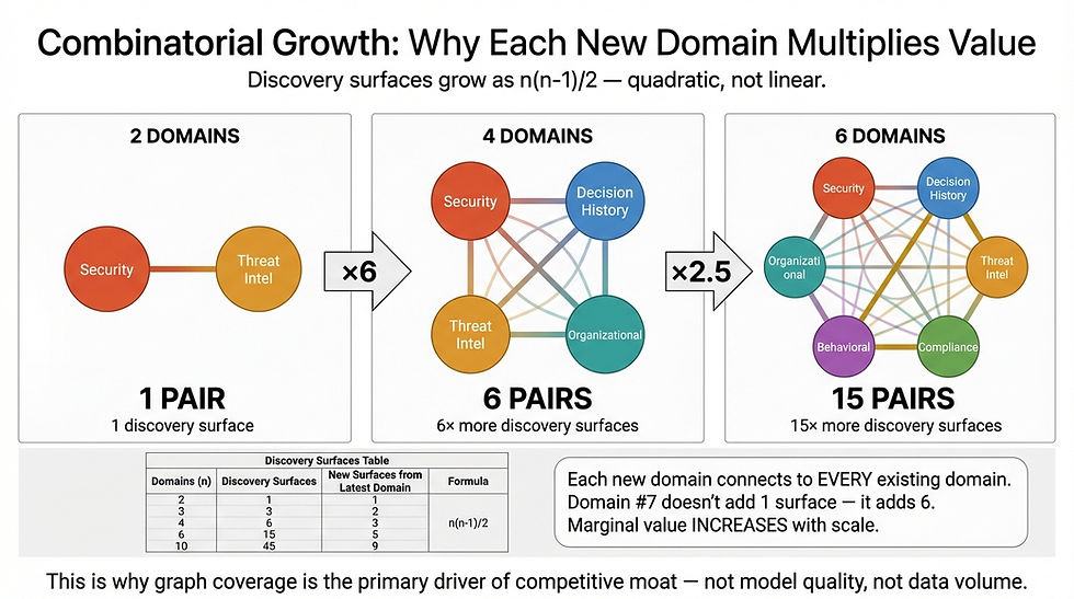
[GRAPHIC #9 | GM-02 | Cross-Graph Connections: Combinatorial Growth (2→4→6 Domains) | The Mechanism: Cross-Graph Attention]

Each new domain adds attention heads with every existing domain. The marginal value of each new domain increases. This is why graph coverage is the primary driver of discovery potential.

The Math Across the Stack: Which Equation Lives Where

The cross-graph attention framework is not one monolithic computation — it is a set of equations distributed across all four layers of the architecture, each executing in a different loop. Understanding the distribution clarifies why you need all four layers to produce compounding intelligence, and why any partial implementation creates an open loop.

Equation	What It Computes	Layer	Loop	What Breaks Without It
Eq. 4: P(action|alert) = softmax(f · Wᵀ / τ)	Alert factor vector f attends to action weight profiles W. Produces action probability distribution.	ACCP — Situation Analyzer	Loop 1 (within each decision)	Agent follows scripts. No situation analysis. No decision economics. Clock 3 never starts.
Eq. 4b: W[a,:] ← W[a,:] + α · r(t) · f(t) · δ(t)	Weight update from verified outcome r(t). Calibrates W to firm's risk profile over hundreds of decisions.	Agent Engineering — AgentEvolver	Loop 2 (across decisions)	W stays generic forever. 68% accuracy never becomes 89%. Decision Clock ticks but rubric never calibrates.
r(t) ∈ {+1, −1}; δ(t) = 20× asymmetry (incorrect penalised 20× harder than correct is rewarded)	Asymmetric reward signal from verified outcome. Encodes security-first risk preference into learning dynamics.	ACCP + Domain Copilots	Loop 3 (every decision, continuous)	Loops 1 and 2 update symmetrically — no risk preference embedded. Action Confusion and Oscillation failure modes emerge.
Eq. 4c: W ← (1−ε)·W after every update	Multiplicative decay. Bounds ||W|| and enables controlled forgetting. Half-life ≈ 693 decisions at standard settings.	Agent Engineering	Loop 2 (governance)	Weights grow unbounded. Treadmill Effect emerges when forgetting rate ε approaches learning rate α.
Eq. 6: CrossAttention(Gᵢ,Gⱼ) = softmax(Eᵢ·Eⱼᵀ/√d)·Vⱼ	Cross-graph discovery sweep. Domain i attends to domain j. Produces enriched embeddings and [:CALIBRATED_BY] write-backs.	UCL — Meta-Graph (Write Source 3)	Cross-graph enrichment (periodic)	Insight Clock never starts. Graph accumulates decisions but never discovers cross-domain connections.
Eq. 9: MultiDomainAttention across n(n−1)/2 pairs	Full multi-domain sweep. 6 domains = 15 attention heads, each discovering a different insight category.	UCL — Meta-Graph	Cross-graph enrichment (periodic)	Only pairwise discovery available. Recursive enrichment — discoveries enabling further discoveries — is absent. Power law is n¹ not n^2.30.

The critical insight: Eq. 6 requires UCL to be meaningful. The cross-attention operation Eᵢ·Eⱼᵀ computes dot products across embeddings from different graph domains. For this to produce discoveries rather than noise, the embeddings must be comparable — they must live in the same semantic space with consistent scaling. UCL enforces this through shared entity definitions, z-score normalisation per feature dimension, and L2 normalisation per entity vector. Without UCL's governed substrate, high dot-product scores between domains reflect scale mismatches, not genuine semantic relationships. UCL is the mathematical precondition for cross-graph attention to work.

Three Properties That Make the Moat Mathematical

The attention framework produces three structural properties — derivable from the interaction geometry — with direct competitive implications. The experiments (Section 10) quantify how strongly they manifest under realistic noise and embedding quality

[GRAPHIC #10 | CGA-03 | Three Properties from Attention Theory | Three Properties That Make the Moat Mathematical]

Property 1: Quadratic Interaction Space

Each domain pair computes mᵢ × mⱼ relevance scores. Total interactions grow quadratically with both the number of domains and the richness of each domain.

Domains connected	Discovery pairs	Total comparisons (at m = 200 entities per domain)
2	1	40,000
4	6	240,000
6	15	600,000
7	21	840,000

The implication: going from 6 to 7 domains adds 240,000 new comparisons — a 40% increase from a single addition. This is a network effect operating at the knowledge layer.

Property 2: Constant Path Length — O(1)

Any entity in any domain attends to any entity in any other domain in a single operation. No intermediate hops. The Singapore threat intel directly enriches the Singapore false-positive pattern — plus 150,000 other comparisons in the same operation.

The business implication: this isn't about speed — it's about coverage. The Singapore connection might be obvious to a senior analyst. But the dozens of other high-relevance pairs in that same sweep — the ones connecting compliance audit schedules to behavioral anomalies to organizational restructuring — those are discoveries no human would make.

Property 3: Residual Preservation — The System Never Forgets

Enrichment is additive: Eᵢ{enriched} = Eᵢ + Σ CrossAttention(Gᵢ, Gⱼ). Every discovery adds to the graph without deleting existing knowledge. With gated residuals and versioned graph snapshots, the system retains access to everything it has learned.

The graph persists through model transitions. When GPT-5 replaces GPT-4, when you swap Claude for Gemini, the accumulated discoveries, calibrated weights, and institutional knowledge are untouched. The moat is in the graph layer, not the model layer.

The competitive advantage isn't locked to any model provider. It's locked to the firm's operating history — which the firm owns, which no vendor can take, and which no model transition can erase.

The Compounding Flywheel

Three properties explain why the moat is super-linear. One mechanism explains why it never stops: the compounding flywheel. Each stage of the cycle produces an output that amplifies the next stage's input. There is no equilibrium. The loop accelerates.

[GRAPHIC #36 | FLYWHEEL | The Compounding Flywheel: Five Stages That Reinforce Each Other | The Compounding Flywheel]

•       Stage 1 — Enriched Graph: UCL ingestion (Write Source 1) and past cross-graph discoveries (Write Source 3) populate richer entity embeddings Eᵢ. More entities. More relationships. Higher-quality representations. Each cycle adds new dimensions to the factor vector f that Loop 1 uses to score decisions.

•       Stage 2 — Better Decisions: Richer embeddings enable the Situation Analyzer (Loop 1, Eq. 4) to read more context per alert. The factor vector f now includes dimensions that didn't exist at deployment — threat-intelligence risk, role-change sensitivity, compliance-audit override. Each additional factor improves action selection and produces more consistently correct outcomes.

•       Stage 3 — Sharper RL Signal: Better decisions produce more consistently correct outcomes. Domain Copilots verify those outcomes. Loop 3 generates more reliably positive r(t) values. The reward signal becomes a stronger, less noisy learning input — which means Eq. 4b in Loop 2 receives cleaner calibration signal.

•       Stage 4 — Richer TRIGGERED_EVOLUTION: Sharper r(t) drives more precise weight updates via Eq. 4b (Loop 2). The weight matrix W calibrates faster and more accurately to the firm's risk profile. These calibrations write [:TRIGGERED_EVOLUTION] relationships back to the graph — Decision History becomes richer, better structured, more informative for Stage 5.

•       Stage 5 — Deeper Discoveries: A richer Decision History domain means higher-quality embeddings in Eq. 6's Eᵢ matrix. Cross-graph attention computes more meaningful compatibility scores. The discovery threshold surfaces more genuine relationships. Discoveries write back as [:CALIBRATED_BY] relationships (Write Source 3), creating new entities in the Institutional Memory domain that enrich Stage 1 for the next cycle.

Cycle completes: Graph Enriched Further → return to Stage 1.

When the Flywheel Stops

The flywheel has three known failure modes, documented in controlled experiments below. Action Confusion stops Stage 2 — two actions with near-identical profiles cause the system to hedge rather than decide. Over-Correction Oscillation corrupts Stage 3 — a single high-severity wrong decision swings weights hard enough to cause cascading errors before equilibrium is restored. The Treadmill Effect (when forgetting rate ε approaches learning rate α) breaks Stage 4 — the system learns and forgets at the same rate, running the flywheel in neutral.

These failure modes don't exist in Generation 1 or Generation 2 systems — because those systems don't have a flywheel to maintain. Knowing them is the price of admission to Generation 3.

The Moat: Why the Gap Is Permanent

The compounding architecture creates an advantage that isn't just hard to close — it's mathematically guaranteed to widen. Here's why.

[GRAPHIC #11 | CGA-02 | Why the Moat Is Super-Linear: O(n² × t^γ) | The Moat: Why the Gap Is Permanent]

The institution's accumulated intelligence grows as:

I(n, t)  ~  O(n² × t^γ)   where γ ≈ 1.5

The intuitive form: Moat = graph coverage × time × search frequency. More domains, more time, more searches — each multiplies the others.

The formal form: n² (each domain pairs with every other) × t^1.5 (domains get richer over time, which compounds on top of the time dimension). Even a conservative γ of 1.2 creates a moat that no linear model can match.

For business readers: A system that's been running 24 months with 6 domains isn't 2× better than one running 12 months with 3 domains. It's roughly 11× better — 4× from domain coverage doubling (quadratic) × nearly 3× from time compounding at γ=1.5 (2^1.5 ≈ 2.8). This is the mathematical reason that first-mover advantage in compounding intelligence is structural, not just temporal.

For technical readers: n² from n(n-1)/2 cross-graph pairs. t^γ from domain sizes mᵢ growing with t, so cross-graph interaction space grows as mᵢ × mⱼ ≈ t². γ = 2 when all domains grow linearly; γ → 1 for stable domains; practical γ ≈ 1.5. Full three-term derivation: Cross-Graph Attention Math, Section 8.

Note: The reference card below decomposes the moat equation into its constituent terms and introduces a practical diagnostic: the γ test. The left column traces the three structural drivers — coverage (n²), time (t^γ), and their product — showing how each contributes to discovery capacity. The empirical scaling panel shows the measured exponent (α ≈ 2.30) with an explicit qualifier: this value is setup-specific, and the key signal is super-linear growth, not the precise exponent.

The γ test (right column) is the diagnostic that matters for practitioners. When γ > 1 — when improvements are gated, promoted through binding eval gates, verified against outcomes, and recorded with audit trails — the system compounds. When γ ≈ 1 — when insights don’t ship, there’s no verification loop, no promotion record, no rollback readiness — the system accumulates linearly at best. The difference between these two trajectories is the difference between a moat and a stockpile. The production artifacts bar at the bottom (Run Receipt, Eval Report, Promotion Record, Rollback Record) lists the evidence that proves γ > 1 in any given deployment.

[GRAPHIC #11a | MOAT-EQ-01, Compounding Intelligence — The Shape of the Moat, The Moat: Why the Gap Is Permanent]

[GRAPHIC #12 | GM-04-v2 | The Gap Widens Every Month | The Moat: Why the Gap Is Permanent]

First mover at month 24: 24^1.5 = 117 units of accumulated intelligence. Competitor starting at month 12: 12^1.5 = 41 units. Gap: 76 — nearly 2× the competitor's total. At month 36: gap = 99 — still growing.

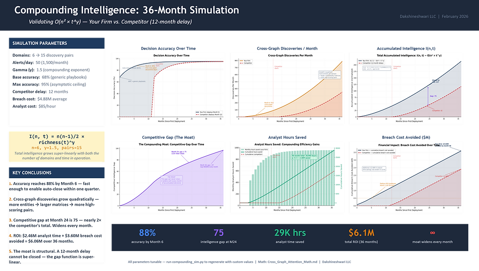
[GRAPHIC #13 | SIM-DASH | 36-Month Simulation Dashboard | The Moat: Why the Gap Is Permanent]

Three reasons the gap can't be replicated:

1. Firm-specific and non-transferable

The Singapore recalibration only matters because your firm had employees traveling to Singapore and your system had been auto-closing those alerts. A competitor running identical code on their infrastructure discovers completely different things — because their organizational structure is different, their threat landscape is different, their behavioral baselines are different. The intelligence is earned from operating experience, not engineered from specifications.

[GRAPHIC #14 | GM-03 | Firm-Specificity of Cross-Graph Intelligence | The Moat: Why the Gap Is Permanent]

2. Temporally irreversible

The discoveries emerged from a specific graph state at a specific moment — 127 accumulated closures + a current threat report + a cross-graph sweep running at the intersection of those two states. The same search tomorrow produces different results because the graph has changed. A competitor can't reproduce it by starting from scratch, even with identical code, because the sequence of decisions and events that created the discovery conditions no longer exists. This isn't a data advantage — it's a trajectory advantage.

3. Model-independent

This is the property that matters most for long-term planning. The graph, the weights, and the discoveries persist through any model transition:

Asset	Survives model transition?
LLM weights	No — lost entirely
Prompt libraries	Partially — may need rewriting
Fine-tuning investment	No — model-specific
Context graph + discoveries	Yes — fully preserved
Scoring weights + calibrated patterns	Yes — operational artifacts, not model artifacts

[GRAPHIC #15 | GM-05-v2 | The Compounding Moat Equation (Dual Form) | The Moat: Why the Gap Is Permanent]

Five Structural Barriers Competitors Cannot Cross

The moat operates on five levels, each reinforcing the others:

Barrier	Why Competitors Can't Replicate
1. Governed context, not per-use-case RAG	Competitors build RAG pipelines per copilot. We build semantic graphs serving every consumer with shared entity definitions. Starting from scratch means rebuilding the entire context layer — months of domain negotiation per customer, not just engineering effort.
2. Meta-graphs for LLM reasoning	Competitors retrieve text chunks by vector similarity. Our cross-graph attention operates on structured semantic embeddings governed by UCL. Without UCL-governed embeddings, Eq. 6 produces noise, not discoveries. The graph topology is the reasoning substrate.
3. Three cross-layer loops, not one	Compounding within decisions (Loop 1), across decisions (Loop 2), governing both (Loop 3: RL Reward/Penalty). Most competitors have zero self-improving loops. Without Loop 3, Loops 1 and 2 learn symmetrically — not security-first. Without Loop 2, Loop 1 never calibrates.
4. Firm-specific discoveries are non-transferable	The Singapore recalibration exists because this firm accumulated 127 decisions while an active campaign emerged. Identical code on a competitor's infrastructure discovers different things. You cannot buy this intelligence. You can only earn it.
5. The gap widens super-linearly	Month 24: 117 units vs. competitor's 41. Gap of 76 — nearly 2× the competitor's total, still growing. By month 36 the gap is 99 and accelerating. Competitors can't catch up by spending more; they can only catch up by also waiting 24 months — and by then, the first mover is at month 48.

Where This Creates Value: Three Verticals

Compounding intelligence isn't a security-specific idea. It applies wherever you have: (a) multiple knowledge domains, (b) recurring decisions, and (c) verifiable outcomes. The math is identical — n domains produce n(n-1)/2 cross-attention heads, each discovering a different category of insight.

The three scenarios below use illustrative timeframes — early months for weight calibration, several months in for cross-graph discovery. Actual trajectories depend on decision volume, domain richness, and the quality of outcome verification. The compounding structure is what matters; the specific months are markers, not milestones.

[GRAPHIC #16 | CI-02 | Cross-Vertical Application: SOC + Supply Chain + Financial Services | Where This Creates Value: Three Verticals]

Scenario 1: Security Operations

The domains: Security Context, Decision History, Threat Intelligence, Organizational, Behavioral Baseline, Compliance & Policy (6 domains, 15 discovery surfaces).

Day 1: The agent follows generic playbooks. Every Singapore login gets the same treatment. Accuracy: 68%.

In early months: The Decision Clock has ticked 340+ times. The weight matrix has calibrated to this firm's risk profile. Decision quality has measurably improved; false negatives are declining.

Later, as the Insight Clock starts ticking: Cross-graph discovery finds: a Singapore credential stuffing campaign invalidates the firm's FP calibration. A CFO promotion changes the risk profile of an account the system has been routinely auto-closing.

The value: At $4.44M average breach cost (IBM 2025), the cross-graph discovery that catches a compromised CFO account pays for several years of the platform in a single event.

[GRAPHIC #17 | CI-VERTICALS-SOC | The SOC Discovery: Three Domains, One Sweep, One Insight No Playbook Contains | Where This Creates Value: Three Verticals]

Scenario 2: Supply Chain

The domains: Supplier Performance History, Procurement Decision History, Geopolitical Risk Intelligence, Demand Forecasts, Logistics & Carrier Data, Financial Health Indicators (6 domains, 15 discovery surfaces).

Day 1: The procurement agent evaluates suppliers against standard criteria — price, lead time, quality score, delivery reliability. Supplier MFG-ASIA-017 scores well on all four. Purchase orders auto-approved.

In early months: The Decision Clock has calibrated. For this firm, lead time variability matters more than average lead time — because their JIT manufacturing process is sensitive to delivery variance, not delivery speed. The weight for lead_time_variance has increased from 0.15 to 0.38.

As the Insight Clock starts ticking: A cross-graph discovery sweep finds three domains intersecting: Supplier Performance History (MFG-ASIA-017 had 3 delivery delays in August-September), Geopolitical Risk Intelligence (monsoon season causes logistics disruptions July-September, this year forecast severe), and Demand Forecasts (Q3 demand projected at 2.3× Q2 — the firm's highest ever).

Discovery:  'The supplier we've been auto-approving for 6 months has a seasonal reliability problem that coincides exactly with our highest-demand period. We're about to put our most critical supply dependency on our least reliable supplier at their worst time of year.' No procurement analyst would have connected monsoon forecasts to demand projections to supplier delivery patterns — the data lives in three different systems managed by three different teams.

The value: A single supply chain disruption at peak demand can cost 5-15% of quarterly revenue. The discovery that triggers early dual-sourcing or inventory buffering prevents a disruption that would have been invisible until it happened.

[GRAPHIC #18 | CI-VERTICALS-SC | The Supply Chain Discovery: Seasonal Risk × Peak Demand × Supplier History | Where This Creates Value: Three Verticals]

Scenario 3: Financial Services

The domains: Trading Decision History, Market Signals & Positions, Regulatory & Compliance Intelligence, Client Profiles & Correspondence, Risk Models, Counterparty Data (6 domains, 15 discovery surfaces).

Day 1: The compliance monitoring agent flags trades that exceed standard thresholds. False flag rate: high.

In early months: The Decision Clock has calibrated. For this firm, equity desk trades in the $5-15M range that stay within sector concentration limits are almost always compliant — 94% of flags in this category were dismissed after review. The weight matrix has learned to suppress these, directing analyst attention to the flags that actually need it.

As the Insight Clock starts ticking: A cross-graph discovery sweep finds four domains intersecting: a new SEC rule (effective in 90 days) restricts certain derivative instruments in 'moderate risk' portfolios; the firm's quant desk has been increasing allocation to exactly those instruments over 4 months; 23% of managed accounts are classified 'moderate risk'; affected instruments represent 12% of total AUM across those accounts.

Discovery:  'A regulatory change effective in 90 days will make 12% of holdings in 23% of our client accounts non-compliant. The position has been building for 4 months — too gradually for any threshold-based alert to catch. Unwinding $340M in positions within 90 days requires careful execution to avoid market impact.' The compliance team didn't catch it because the trades were individually compliant; they only become a problem when you connect the regulatory change, the portfolio drift, and the client classification — three threads in three different systems.

The value: Regulatory fines for this type of violation range from $10-50M. Client lawsuits add another layer. But the real cost is reputational — the kind of headline that costs a wealth management firm 5-10% of AUM as clients move assets. Early discovery turns a crisis into an orderly transition.

[GRAPHIC #19 | CI-VERTICALS-FS | The Financial Services Discovery: Four Domains, One Regulatory Exposure Found Before the Clock Runs Out | Where This Creates Value: Three Verticals]

The Pattern Across All Three

	SOC	Supply Chain	Financial Services
Day 1 problem	Generic alert triage	Generic supplier scoring	Generic compliance flagging
Early phase: calibration	Weights calibrate to firm's risk profile	Weights calibrate to operational sensitivities	Weights calibrate to trading patterns
Later: cross-graph discovery	Singapore threat × FP pattern	Monsoon risk × demand spike × supplier history	Reg change × portfolio drift × client class
Why no human caught it	Data in 3 different dashboards	Data in 3 different teams' systems	Data in 3 different departments
Business value prevented	$4.44M breach	5-15% quarterly revenue loss	$10-50M regulatory action

[GRAPHIC #20 | PATTERN | The Pattern Across All Three Verticals | Where This Creates Value: Three Verticals]

In each case: the system starts generic, calibrates through experience, then discovers cross-domain connections that no single knowledge domain contains. The mathematical structure is identical. The moat equation — I(n, t) ~ O(n² × t^γ) — applies to all three. The judgment compounds. The gap widens. The advantage is permanent.

The architectural bet isn't vertical-specific. It's that institutional memory compounds — and the system that starts accumulating it today has a moat that begins widening the moment the first discovery fires.

Why Current AI Security Approaches Don't Compound

The market for AI in security operations has exploded. Gartner added 'AI SOC Agents' to the 2025 Hype Cycle. IDC tracks 40+ vendors. Every major platform is bolting AI onto existing products. But the market has split into three generations — and understanding the difference is the key to knowing which investments compound and which depreciate.

[GRAPHIC #21 | CI-GENERATIONS | Three Generations of SOC AI | Why Current AI Security Approaches Don't Compound]

Generation 1: Faster Playbooks

The first wave automated existing SOC workflows. SOAR platforms, hyperautomation tools, no-code orchestration engines — vendors such as Torq HyperSOC, Cortex XSOAR, and Swimlane made playbooks run 5× faster with parallel execution and pre-built integrations.

The problem: playbooks are static logic. When threat actors change tactics, someone rewrites the playbook. The system on Day 365 has exactly the same decision-making capacity as Day 1 — it just executes faster.

Characteristic: Fast execution. Static intelligence. Humans maintain the logic. No learning.

Generation 2: AI Analysts

The second wave deployed autonomous AI agents that can investigate alerts, gather evidence, reason about findings, and recommend actions. Some offer 'glass box' transparency — replayable investigation timelines showing exactly what was queried and why (Prophet Security). Some deploy in 30 minutes and cost less than a junior analyst (Dropzone AI). Some integrate with existing SIEM and behavioral baselines to provide autonomous response (Darktrace Cyber AI Analyst, 7AI).

The problem: each investigation starts from scratch. Alert #10,000 is investigated with the same knowledge as Alert #1. The agent may learn from feedback to adjust its behavior, but it doesn't accumulate a persistent, traversable layer of institutional intelligence. It doesn't get smarter in a way that compounds.

The diagnostic question to ask any Generation 2 vendor: after 10,000 investigations, show me the compounding curve — how the system's accuracy, speed, and discovery depth have improved over time. Generation 2 vendors cannot answer this, not because their systems aren't capable, but because the architecture doesn't accumulate intelligence across decisions.

Characteristic: Autonomous investigation. Explainable reasoning. No memory across decisions. No compounding. Each alert is fresh.

Generation 3: Compounding Intelligence

The third wave — the architecture described in this paper — connects three capabilities that neither previous generation has:

•       A context graph that accumulates institutional knowledge. Not a static knowledge base configured on day one, and not anomaly baselines per device. A living graph fed by three simultaneous write sources: UCL ingestion from external systems, AgentEvolver [:TRIGGERED_EVOLUTION] relationships from verified decisions, and cross-graph enrichment [:CALIBRATED_BY] relationships from discovery sweeps. Every decision, every outcome, every cross-domain discovery persists and makes the next decision better.

•       Three cross-layer loops that write back to the graph. Not just feedback that adjusts next-response behaviour. Three explicit loops — Loop 1 (Situation Analyzer: smarter within each decision), Loop 2 (AgentEvolver: smarter across decisions), and Loop 3 (RL Reward/Penalty: governs both other loops with asymmetric reinforcement, continuous, every decision) — all three writing verified intelligence back to the shared context graph.

•       Decision economics that translate every action into measurable business impact. Not 'we resolved 500 alerts.' Instead: '$127 cost avoided per auto-close, 44 analyst-minutes saved, 0.003% residual risk accepted.' CFO-readable. Per decision.

Remove any one of these three, and intelligence stops compounding:

•       Context graph without learning loops = a database (rich, but static)

•       Learning loops without a context graph = improvement without memory (the agent gets better but can't explain why or share what it learned)

•       Either without decision economics = undifferentiated AI spend (the CFO can't distinguish your system from any other vendor's)

Characteristic: Self-improving judgment. Compounding moat. Three cross-layer loops feeding one living graph. The gap widens automatically.

[GRAPHIC #22 | CI-TRIANGLE | What Makes Intelligence Compound? | Why Current AI Security Approaches Don't Compound]

The structural comparison below makes the generational divide concrete. The top three rows — alert triage automation, autonomous investigation, and explainable decisions — are table stakes. Every serious vendor in 2026 delivers these. The compounding layer (rows 4-9) is where Generation 3 separates architecturally from the rest. No vendor delivers the compounding layer by adding AI to an existing product. It requires the graph, the loops, and the economics — designed together from the start.

[GRAPHIC #23 | CI-MATRIX | What Compounds vs. What Doesn't (4-col structural view) | Why Current AI Security Approaches Don't Compound]

The vendor landscape below maps these same structural capabilities against specific players in the current AI SOC market — from platform copilots and behavioral baseline systems through agentic triage startups and hyperautomation engines. Every vendor in the matrix delivers rows 1-3 (table stakes). Zero deliver rows 4-9 (the compounding layer). The rightmost column is the architectural target.

[GRAPHIC #24 | CI-COMPETE-MATRIX | SOC AI Capability Landscape (7-col vendor view) | Why Current AI Security Approaches Don't Compound]

Experimental Evidence for Compounding

The architecture described above makes specific, testable predictions. We recently validated the mathematical framework through four controlled experiments using synthetic SOC data. Here are the headline results.

The Scoring Matrix Learns

The decision-making component — a 6-factor × 4-action scoring matrix with temperature-controlled softmax — was initialized with random weights and fed 5,000 synthetic alerts with known ground-truth optimal actions. The system learned online, updating its weight matrix after each decision using asymmetric reinforcement (failures penalized 5× harder than successes are rewarded, reflecting the reality that a missed threat is far more costly than an unnecessary escalation).

Result: The system converged to 69.4% accuracy from a 25% random baseline, with a clear three-phase learning curve — random exploration (decisions 0-200), rapid calibration (200-1500), and diminishing returns (1500-5000) as remaining errors reflected genuinely ambiguous alerts.

This is the Decision Clock ticking. Same system. Same factors. Evolved weights. The 68% → 89% trajectory described in the architecture is consistent with what the controlled experiment shows — production accuracy is higher because real alert distributions have more structure than synthetic data.

[GRAPHIC #25 | EXP1-BLOG | Scoring Convergence Curve (Experiment 1) | Experimental Evidence for Compounding]

Cross-Graph Discovery Is Real and Measurable

We created two synthetic graph domains — Security Context (100 entities) and Threat Intelligence (80 entities) — with 15 'planted' true discoveries: entity pairs that share semantic attributes a domain expert would flag as related. Then we ran cross-graph attention and measured how many true discoveries it found.

Result: With properly normalized entity embeddings, the cross-graph attention mechanism discovered true relationships at 110× above random baseline (F1 = 0.293). Without normalization, performance dropped to 23× — still far above random, but dramatically weaker.

The implication: cross-graph discovery isn't a metaphor. It's a measurable architectural capability. And embedding quality — how well entities are represented in the shared vector space — is the critical prerequisite. This is the technical reason UCL's normalisation step matters.

[GRAPHIC #26 | EXP2-F1 | Cross-Graph Discovery: 110× Above Random Baseline (Experiment 2) | Experimental Evidence for Compounding]

Discovery Scales Super-Quadratically

The most striking experimental finding: when we varied the number of graph domains from 2 to 8, the number of discoveries followed a power law:

D(n) ∝ n^2.30    (R² = 0.9995)

This is steeper than quadratic. Each new graph domain contributes more discoveries than the last — because discoveries from one domain pair create enriched entity representations that make discoveries in other domain pairs more likely. Discoveries catalyze further discoveries.

The exponent (2.30) is empirical for this experimental setup — production values will depend on domain quality, alignment strength, and graph density — but the structural point holds: discovery capacity grows faster than linearly, and each additional domain contributes more than the last.

This is the mathematical basis for the moat: the gap between a system with 6 connected domains and one with 3 isn't 2× — it's closer to 5×. And this multiplies with operating time.

Compounding is not a metaphor. It is a measurable property of the architecture.

For the full mathematical framework, experimental details, and sensitivity analysis, see the companion paper: Cross-Graph Attention: Mathematical Foundation.

[GRAPHIC #27 | EXP3-BLOG | Discovery Scaling with Graph Coverage (Experiment 3) | Experimental Evidence for Compounding]

What Breaks the System — and When

The fourth experiment asked: how sensitive is the architecture to its own parameters? Four sweeps varied the asymmetry ratio, the softmax temperature τ, the noise rate in alert labels, and the embedding dimensionality.

Two findings with direct production implications:

•       Noise is the critical threat. Accuracy holds stable up to about 5% label noise, then degrades sharply. Above 10% noise — meaning 1 in 10 verified outcomes is wrong — the system's learning signal corrupts faster than it accumulates. This is the phase transition. In practice, outcome verification quality matters more than any other parameter. A system with noisy feedback learns to be wrong.

•       Embedding dimension has a sweet spot — and a cliff. Performance peaks at d=128 for the experimental setup. At d=256, discovery collapses entirely (F1=0): the model is over-parameterized for the available signal, and the attention mechanism finds noise instead of true relationships. Bigger is not better. Match embedding size to the actual richness of the domain data.

[GRAPHIC #28 | EXP4-SENS | Parameter Sensitivity Analysis: Noise Threshold and Embedding Sweet Spot (Experiment 4) | What Breaks the System — and When]

Three Failure Modes Every Enterprise Should Know

The experiments didn't just validate the architecture — they revealed three systematic failure modes that any enterprise deploying AI that learns from its own decisions needs to understand. These aren't bugs. They're structural properties of online learning systems. Knowing them is the difference between a system that gets smarter and one that oscillates or stalls.

Failure Mode 1: Action Confusion

When two possible actions have similar profiles — both triggered by similar alert characteristics — the learning system struggles to distinguish them. The result: the system hedges, assigning near-equal probability to both actions, effectively deferring the decision.

What to do about it: Design action sets with maximally distinguishable profiles. If 'escalate to Tier 2' and 'enrich and wait' are often interchangeable, either merge them or add a factor that discriminates (e.g., 'analyst capacity available right now').

Failure Mode 2: Over-Correction Oscillation

When the system penalizes missed threats more heavily than unnecessary escalations (which it should — a missed threat can cost millions), a single bad outcome can swing the weights hard enough to cause several subsequent false escalations. Those are then corrected at normal strength, creating a damped oscillation that wastes 200-300 decisions worth of learning signal.

What to do about it: Tune the asymmetry ratio to the domain. High-consequence domains (SOC, anti-money laundering) justify 5-10× asymmetry. Lower-consequence domains (IT service management, helpdesk) can use 1.5-2× for smoother convergence.

Failure Mode 3: The Treadmill Effect

The system needs to balance learning (incorporating new outcomes) with stability (retaining what it's already learned). If the forgetting rate is too close to the learning rate, new knowledge is partially erased before it consolidates. The system runs on a treadmill — always learning, never accumulating.

What to do about it: Monitor the learning-to-forgetting ratio. The optimal ratio (~20:1) should increase for stable environments (where forgetting is harmful) and decrease for rapidly shifting threat landscapes (where adaptability matters more than consolidation). A rising false-positive rate after a stable period is an early indicator that the environment has shifted and the forgetting rate may need adjustment.

Why This Matters Competitively

These failure modes are invisible to systems that don't learn from their own decisions. If your AI SOC tool processes each alert from scratch, it never encounters action confusion, oscillation, or the treadmill effect — because it never accumulates weights in the first place. These are problems only compounding systems have. And knowing them is the price of admission to Generation 3.

[GRAPHIC #29 | CI-FAILUREMODES | Three Failure Modes of Self-Improving AI | Three Failure Modes Every Enterprise Should Know]

The Widening Gap

Here is why the choice of architecture matters more than the choice of vendor.

Consider two organizations that deploy AI in their SOC on the same day. Organization A deploys a Generation 2 system — an autonomous AI analyst that investigates each alert intelligently but independently. Organization B deploys a Generation 3 system — compounding intelligence with a context graph, three learning loops, and decision economics. The following illustrates how the gap opens over time; specific timeframes will vary by deployment.

At deployment: Both handle Tier 1 triage. Performance is similar — perhaps Organization A's system is even faster out of the box, since it's optimized for single-alert investigation speed.

After several months: Organization B's system has processed thousands of alerts. Its context graph contains validated decision traces, evolved scoring weights, and cross-graph discoveries (like the Singapore recalibration). Its auto-close accuracy has risen from 68% to 89%. Organization A's system has also processed thousands of alerts — but each one from scratch. Its accuracy is the same as on day one.

Within the first year: Organization B adds a second specialist copilot (e.g., for insider risk). It inherits the full context graph on day one — every pattern, every decision trace, every cross-domain insight. It starts smart. Organization A adds a second tool. It has no shared intelligence layer. It starts from zero.

As the system matures: Organization B has multiple copilots sharing a rich context graph. Our experiments show that discovery capacity scales as n^2.30 with the number of connected domains — so three copilots don't find 3× the insights, they find closer to 10×. Organization A has multiple independent tools. Each is individually capable. None makes the others smarter.

The gap doesn't close. It widens.

This is the mathematical structure of compounding applied to institutional knowledge. It's not a linear advantage that competitors can close by running faster. It's a super-linear advantage that accelerates with every month of operation and every domain connected.

The test is simple: ask whether your system's reasoning on a given alert will be different in six months than it is today. If the answer is no — if Day 180 looks identical to Day 1 — the system doesn't compound. Every dollar spent on it is an operating expense, not a capital investment.

[GRAPHIC #30 | CI-WIDENINGGAP | Two Architectures, 24 Months Apart | The Widening Gap]

The Platform Pattern

The architecture described in this paper — context graph + three learning loops + decision economics — is not specific to security operations. The same pattern applies wherever enterprise AI makes repeated decisions that should get better over time:

•       Source-to-Pay: Price variances, PO exceptions, vendor risk assessments. The graph accumulates contract terms, pricing patterns, and supplier reliability. Decisions about procurement get smarter. Projected impact: COGS savings compounding quarterly.

•       IT Service Management: Incident tickets, change requests, SLA monitoring. The graph accumulates service dependencies, resolution patterns, and escalation histories. Triage gets faster. Root cause identification gets more accurate.

•       Anti-Money Laundering: Transaction alerts, customer risk profiles, regulatory filings. The graph accumulates entity relationships, transaction patterns, and investigation outcomes. False positive rates decline. SAR quality improves.

In each domain, the diagnostic question is the same: does the system get measurably better at its job over time? If yes, the architecture is compounding. If no, it's automation — valuable, but not a moat.

The competitive moat is not in any single domain. It's in the architectural pattern that makes intelligence compound — and in the graph that accumulates across domains once you connect them.

Implications

For CISOs and Security Leaders

The question isn't 'which AI vendor has the best model?' Models are commoditizing. The question is: which architecture accumulates institutional knowledge that makes every future decision better?

Ask your vendor: 'If I run the same alert through your system today and six months from now, will the reasoning be different?'

Answer	Clock	What it means
'The reasoning will be identical'	Clock 1-2	Tool. No compounding. Day 1 = Day 180.
'We'll retrain/fine-tune with new data'	Clock 1	Improvement requires vendor cycles. Not self-improving.
'The context graph will be richer'	Clock 2	Better recall, same reasoning.
'The weights will have calibrated to your risk profile'	Clock 3	Self-improving judgment earned through experience.
'The system will have discovered cross-domain patterns'	Clock 4	Full compounding intelligence.

The procurement implication: every dollar on a Clock 1-2 system is an operating expense — it buys the same capability forever. Every dollar on a Clock 3-4 system is a capital investment — it buys compounding capability that appreciates with use.

[GRAPHIC #31 | FC-06 | Four Clocks Comparison Table | Implications]

For Investors and Strategic Decision-Makers

Traditional AI metrics measure capability at a point in time. The metrics that matter for compounding intelligence measure the rate of self-improvement:

Metric	What It Measures	Why It Matters	Benchmark
Decision improvement rate	Accuracy gain per N decisions	Proves the system learns	>0.5% per 100 decisions (illustrative)
Cross-graph discovery rate	New connections per search cycle	Proves cross-domain value	>2 discoveries/day once Insight Clock active
Pattern creation rate	Autonomously created patterns/month	System expands its own criteria	>5 patterns/month once Insight Clock active
Re-run lift	Improvement on historical decisions	Backward-looking quality gain	>10 points on decisions 30+ days old

The valuation lens: Clock 1-2 AI = software (SaaS multiples). Clock 3-4 AI = platform with network effects (increasing returns to scale). The switching cost isn't contractual — it's the loss of accumulated judgment that took months to develop.

The due diligence test: ask the company to run its oldest available alert through the current system and through a snapshot from six months prior. If the decision, confidence score, and contributing factors differ — the system compounds. If they're identical, you have automation priced as a platform.

[GRAPHIC #32 | INDUSTRY | Enterprise AI Waves: From Models to Compounding Systems | Implications]

For the Industry

The first wave of enterprise AI (2023-2025) was about making models useful — RAG, fine-tuning, guardrails, orchestration. It created value but not defensibility.

The second wave (2026+) is about systems that learn from their own operation. The defensibility comes from accumulated, firm-specific judgment that emerges from running the system in production over months and years.

The architectural pattern is clear: four dependency-ordered layers (UCL, Agent Engineering, ACCP, Domain Copilots) enable three cross-layer loops that feed one living graph. The mathematical framework — cross-graph attention applied to institutional knowledge — provides the formal foundation. The properties are proven. And the central insight is expressible in a single sentence:

Transformers let tokens attend to tokens. We let graph domains attend to graph domains. Same math. Applied to institutional judgment instead of language.

[GRAPHIC #33 | CI-05 | The Rosetta Stone: Transformers ↔ Cross-Graph Attention | Implications]

The moat isn't the model. The moat isn't the agent. The moat is the graph — and the graph develops judgment.

This paper draws on the mathematical framework formalized in Cross-Graph Attention: Mathematical Foundation, which provides the complete derivation with shape-checked equations, worked examples, and LLM judge review. Four controlled experiments validate the framework: scoring matrix convergence (69.4% accuracy), cross-graph discovery (110× above random), super-quadratic scaling (b = 2.30, R² = 0.9995), and sensitivity analysis with phase transitions. The SOC Copilot demo — a working proof-of-concept — demonstrates Clocks 1-3 in production.

Companion reading: Gen-AI ROI in a Box  ·  Unified Context Layer (UCL)  ·  Enterprise-Class Agent Engineering Stack  ·  Cross-Graph Attention: Mathematical Foundation

Arindam Banerji, PhD  ·  banerji.arindam@gmail.com  ·  Dakshineshwari, LLC